Laser Pulse Characterization
Pulsed lasers can achieve large peak powers by squeezing the energy of a pulse into a small duration of time. This enables applications requiring high intensities such as laser processing and nonlinear frequency conversion. Furthermore, ultrashort pulses are critical for probing fast light-matter interactions and for high-speed optical communications. As a result, accurate temporal characterization of pulsed sources is as critical as accurately estimating the pulse energy and spatial and spectral profiles. As discussed in Methods for Pulsed-Laser Operation, techniques can lead to pulse durations ranging from µs to fs. Direct measurements of pulses less than 20 ps using photodetectors remain a challenge as the response time of high-speed photoreceivers is currently limited to 10 ps (see Types of Photoreceivers). Consequently, indirect methods for measuring ultrashort pulses using optical gating techniques have been developed and are discussed below. Prior to addressing the characterization techniques, attributes of a pulse laser’s temporal profile are detailed.
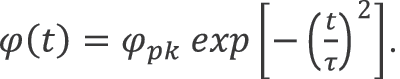
For a pulsed laser, the output power (φ) is a time-dependent quantity. Like the laser beam spatial profile discussed in Laser Beam Spatial Profile, the temporal profile has both an amplitude, a pulse shape, and a width. One common profile takes the shape of a Gaussian function (as shown in Figure 1) and can be written as follows:
Laser Pulse Temporal Profile
The pulse width . is defined as the radius (HW1/e) at which the power decreases to 1/e or 0.37 of its peak power (φpk) value. The temporal width is sometimes reported as its FWHM value, which—for a Gaussian pulse—is larger than . by a factor of 2(ln2)1/2. Laser systems can produce many pulse shapes, including a Lorentzian, hyperbolic secant, as well as a flat-top. Similar to laser beams, laser pulses can undergo modification following propagation. One important consequence of this modification is that ultrashort pulses, i.e., values of τ less than 35 fs, can experience significant pulse broadening in dispersive media after propagation of only a few centimeters.
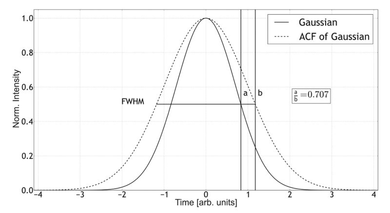
Figure 1. A Gaussian temporal pulse function and its normalized autocorrelation function (dotted line).
The value of .pk is distinctly different from the average power since it gives the instantaneous value of the power at the peak of the pulse. The value of .pk for a Gaussian pulse can be determined by recalling from Equation (8) that integration of φ(t) over the entire pulse gives the pulse energy (Qe). Therefore, by integrating the Gaussian pulse in the above equation, one can obtain the peak power, i.e., φpk = Qe/τ√π, where the inverse relationship between peak power and pulse width is clear. Furthermore, by taking this Gaussian form of φ(t) and inserting it into the irradiance distribution for a Gaussian beam given, the spatiotemporal irradiance distribution for a pulsed laser is generated. Such a formula is critical for estimating important quantities such as peak irradiance or peak power density.
Measurement of a temporal event requires that the response of the detection method be at least as fast as the event being measured. Since response times of high-speed photoreceivers are limited, measurement of a pulse with sub-10 ps duration relies on the optical pulse itself to act as the response function. An autocorrelator is a device (see Figure 2) that utilizes this approach for measuring the pulse shape and duration of ultrafast laser pulses. Autocorrelation is the simplest method for determining pulse widths when phase information of the pulse is not required (see below for a more comprehensive approach). Autocorrelation is based on recording the second order correlation function using a Michelson interferometer (see coherence portion of Laser Light Characteristics for details about the interferometer). An incoming pulse with electric field E(t) is first split into two replicas by means of a beamsplitter. The replicas are sent down two independent temporal delay lines, one variable and one fixed, to generate a time delay between them. Then, the two replicas, E(t) and E(t-τ), are recombined in a nonlinear crystal to produce SHG (see Laser Spectral Tunability for details). The total intensity of the SHG signal is proportional to the square of the sum of the fields as shown in Figure 2. There is a component of the signal ([2E(t)E(t-τ)]) that is due solely to the temporal overlap of the two pulses. This component of the signal will only be present when the two pulses are overlapping in time. An iris or aperture allows only this component to be sent to a detector, typically a photodiode. The photodiode squares the signal and integrates it, giving an intensity proportional to the intensity of the two replicas. By recording this signal as a function of the time delay, the intensity autocorrelation of the laser pulse is generated.
Autocorrelation
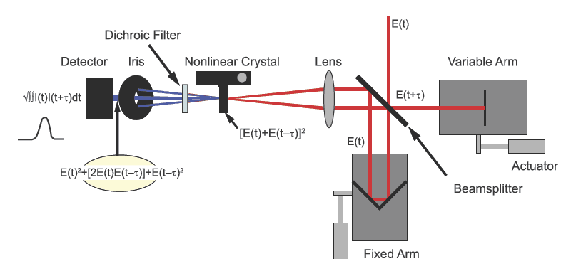
Figure 2. Schematic of a typical autocorrelator.
The equation for the autocorrelation shown on the left side of Figure 2 is a correlation function of the two replicas and not a direct measurement of the pulse. If the two replicas are identical, this equation can be solved analytically and the pulse width can be determined simply by dividing the autocorrelation signal width by a constant factor that depends on the profile of the pulse. It should be clear that the autocorrelation width is always greater than the width of the actual pulse. This can be seen for the Gaussian pulse shown in Figure 1, where the autocorrelation width is a factor of √2 larger than the pulse width.
Because of the time-bandwidth uncertainty principle, ultrashort laser pulses carry significant spectral bandwidth (typically from 10 to 100 nm). Autocorrelation can measure the duration of an ultrashort pulse, but it is unable to characterize the phase relationship between the different constituent spectral components. The primary reason for this is that autocorrelators utilize a single element photodetector that effectively integrates over the spectral profile of the pulse. The relationship between the spectral components of light can change upon propagation in a dispersive medium leading to an effect known as chirp, which can cause pulse broadening. Fortunately, techniques exist that monitor the spectral profile of a pulse as a function of time, allowing for complete reconstruction of the electric field. Of these techniques, Frequency-Resolved Optical Gating (FROG) is arguably the most straightforward and easiest to implement. Figure 3 shows the simplest version of this technique (SHG FROG) which is essentially a spectrally-resolved autocorrelator that sends the SHG signal into a spectrometer instead of a single element photodiode. Figure 3 shows typical signals (called traces) generated from a SHG FROG set-up and reveals the impact of pulse broadening following propagation in a dispersive medium. Extracting the electric field from a FROG trace, known as a retrieval, is significantly more complicated than extracting the intensity from an autocorrelation signal. Analysis of FROG traces requires an iterative method incorporating a two-dimensional phase retrieval algorithm. Fortunately, efficient algorithms for phase retrieval exist. There are alternative geometries that can be used for FROG, including the Self-Diffraction FROG (SD FROG). This geometry provides the sign of the spectral phase (not extracted using a single SHG FROG scan) and is more intuitive to analyze, allowing for chirp measurements to be made in real time. The downside is that SD FROG relies on very high peak powers to generate sufficient signals.
Frequency-Resolved Optical Gating
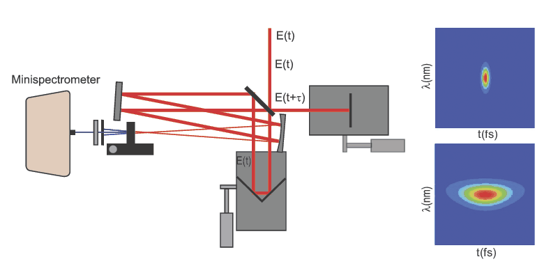
Figure 3. Schematic of a SHG FROG set-up (left) and SHG FROG traces (right) for a 20 fs pulse before (a) and after (b) traveling through a dispersive medium.
Related Topics
Light-Matter Interactions in Lasers Critical Laser Components Characteristics of Laser Light Types of Lasers Methods for Pulsed-Laser Operation Radiometric Measurement Thermopile Sensor Physics Pyroelectric Sensor Physics Photodiode Sensor Physics LED Characterization Laser Beam Spatial Profiles Laser Beam Profile Measurement

For additional insights into photonics topics like this, download our free MKS Instruments Handbook: Principles & Applications in Photonics Technologies
Request a Handbook