Pulsed Radiation
Here we briefly cover radiation of varying level. This requires consideration of the dependence on t, time, so that irradiance becomes Eeλ (λ,t). Most displays of radiation pulses show how the radiant power (radiant flux) Φe(λ,t) varies with time. Sometimes, particularly with laser sources, the word “intensity” is used instead of radiant flux or radiant power. In this case, intensity often does not represent the strict meaning indicated in Table 1, but beam power.
Single Pulse
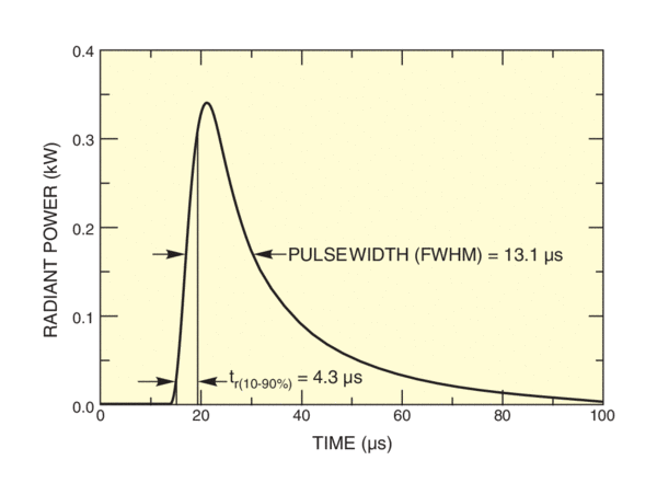
Figure 1 shows a typical radiation pulse from a flash lamp or laser. Microsecond timescales are typical for flashlamps, nanosecond timescales are typical for Q-switched or fast discharge lasers, and picosecond or femto-second timescales are typical of mode locked lasers. Pulse risetimes and decay times often differ from each other, as the underlying physics is different.
The pulse shape shows the dependence of radiant power, with time. The radiant energy in a pulse is given by:
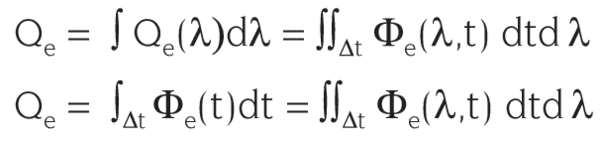
Φe(λ,t) represents the flux per unit wavelength at wavelength λ and time t; Φe(t) represents the total flux (for all wavelengths), at time t. Φe(λ) is the spectral distribution of radiant energy, while Qe represents the total energy for all wavelengths.
For Φe(t) in Watts, Qe will be in joules.
Δt, is the time interval for the integration that encompasses the entire pulse, but in practice it should be restricted to exclude any low level continuous background or other pulses.
The pulse is characterized by a pulsewidth. There is no established definition for pulsewidth. Often, but not always, it means halfwidth, full width at half maximum (FWHM). For convenience average pulse power is often taken as the pulse energy divided by the pulsewidth. The validity of this approximation depends on the pulse shape. It is exact for a “top hat” pulse where the average power and peak power are the same. For the flashlamp pulse shown in Fig.1, the pulse energy, obtained by integrating, is 6.7 mJ, the pulse width is 13.1 µs, so the “average power” computed as above is 0.51 kW. The true peak power is 0.34 kW and thus a nominal inconsistency due to arbitrary definition of pulse width.
Repetitive Pulses
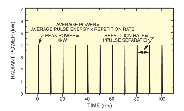
Figure 2 shows a train of pulses, similar to the pulse in Fig. 1. Full characterization requires knowledge of all the parameters of the single pulse and the pulse repetition rate. The peak power remains the same, but now the average power is the single pulse energy multiplied by the pulse rate in Hz.
Tech Note
When recording pulses you should ensure that the detector and its associated electronics are fast enough to follow the true pulse shape. As a rule of thumb, the detection system bandwidth must be wider than 1/(3tr) to track the fast risetime, tr, to within 10% of actual. A slow detector system shows a similar pulse shape to that in Fig.1, but the rise and fall times are, in this case, characteristic of the detector and its electronic circuitry. If you use an oscilloscope to monitor a pulse you will probably need to use a “termination” to reduce the RC time constant of the detection circuitry and prevent electrical signal reflections within a coaxial cable. For example, an RG 58/U coaxial cable requires a 50 ohm termination.