Solar Simulator Sample Calculations

The spectral irradiance at any wavelength, E_λ, is in units of watts per square meter per nm (W m-2 nm-1). The value is a measure of the flux per nm at the specified wavelength incident normally onto an element of the surface divided by the area of the surface element in square meters. The value can be expressed in other units such as W cm-2 nm-1 or W m-2 µm-1. For example, 1.23 W m-2 nm-1 is equivalent to 0.000123 W cm-2 nm-1 or 0.123 W cm-2 µm-1.

If a beam of irradiance E_λ (W m-2 nm-1) falls on a sample of area A square meters, the total irradiance on the sample will be A E_λ (W nm-1).

The total irradiance between two wavelengths λ₁ and λ₂ is equal to the integral of the E_λ curve between λ₁ and λ₂. This is the area of the curve between λ₁ and λ₂ and the units will be in W m-2. Our simulator spectral irradiance curves include tabled values of the percentage of the total radiation. We compute the data for these tables and the total irradiance, using trapezoidal integration of our measurement data. The data is a series of discrete irradiance/wavelength pairs. These tables allow you to calculate the irradiance for any wavelength ranges coinciding with the tabulated values.

Since the curves also include the total irradiance for each simulator beam size, you can find the irradiance for tabulated wavelength ranges for any of our simulators.

If you need to estimate the total irradiance in a wavelength interval not bounded by the tabulated values then you can use simple geometry to calculate the area under the curve for your wavelength interval.

To find the total radiation dose within a specified wavelength range you first need to compute the irradiance for this wavelength interval. The result will be in W m-2. When you multiply this by the exposure time in seconds the result is the dose in J m-2 (joules per meter squared). When you multiply this by the sample area, you get the total dose on the sample. Note that you must use the sample area in square meters.

To find the effective dose you need to know the action spectrum for the effect and convolve this with the simulator spectrum. You then integrate the convolved spectrum. For absolute data, you will need the absolute action spectrum; the relative spectrum is adequate to compare simulators with solar spectra.

Find the irradiance in the wavelength range 450 - 700 nm from a 91191, 2 x 2 inch kW simulator with AM 1.5 Global Filter.

Step 1: Find what fraction of the output is in the specified range. (Figure 2 shows the tabled data.) The total percentage of the output in this range = 47.4%

Step 2: Multiply the fraction by the total power.

The top table in Figure 2 shows the total output power density to be 7150 W m-2 for this model. Therefore the irradiance for the 450 - 700 nm range is:

0.474 x 7150 = 3389 W m-2

Determine the total 680 - 720 nm radiation dose on a 2 cm2 sample in the work plane of the AM 1.5 D simulator with irradiance curve shown in Figure 3 when the shutter is opened for 1.5 minutes.

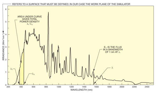
Step 1: Determine the irradiance in the specified spectral region by measuring the area under the curve over the specified wavelength range. We use the curve shown. Note that this curve is for a simulator with a 4 x 4 inch (102 x 102 mm) beam. Our example is for a 2 x 2 inch (51 x 51 mm) beam.

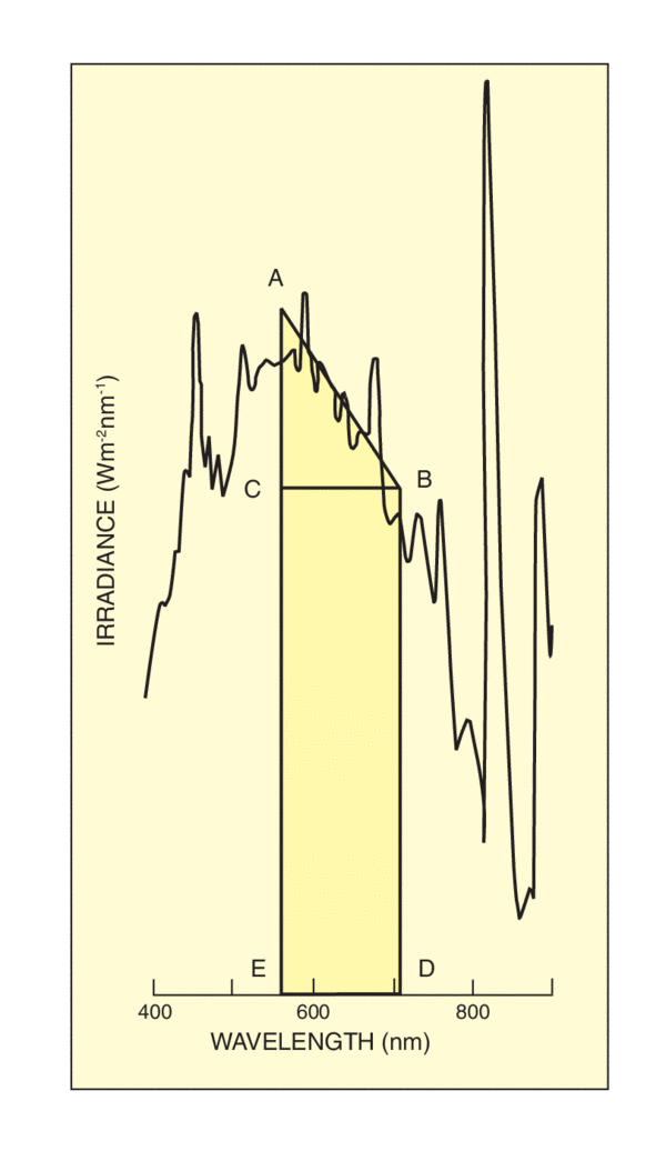
We drew the line AB as best estimate of the average of the curve from 680 - 720 nm. Use a photocopier with magnification to make this area measurement easier. The area under the curve is approximately the sum of the area of the triangle ABC and the rectangle CBDE. We use simple scaling of the axes to find CE, and AC.

Area ABC = 140 x 0.5 x 0.82 = 57.4 W m-2

Area CBDE = 140 x 3.16 = 442 W m-2

Total area, ABC + CBDE, = 499 W m-2

The total irradiance or power density is 499 W m-2 for a 4 x 4 inch simulator. Since our example deals with a 2 x 2 inch model, we must multiply the output by the relative outputs of these two models, i.e. 10360/2765 = 3.75

499 W m-2 x 3.75 = 1871 W m-2

Step 2: Find out how much power falls on the sample.

The irradiated area is 0.02 m x 0.02 m = 0.0004 m2, so the total radiation falling on the sample is

0.0004 m2 x 1871 W m-2 = 0.75 W

Step 3: Calculate the dose, i.e. the total energy that falls on the sample in 1.5 minutes. The dose is the power multiplied by the exposure time, 90 seconds

0.75 W x 90 s = 67.5 J (1 Ws = 1 J)

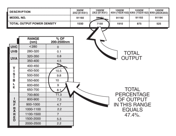
Find the irradiance in the wavelength range 450 - 700 nm from a 91191, 2 x 2 inch kW simulator with AM 1.5 Global Filter.

Step 1: Find what fraction of the output is in the specified range. (Figure 2 shows the tabled data.) The total percentage of the output in this range = 47.4%

Step 2: Multiply the fraction by the total power.

The top table in Figure 2 shows the total output power density to be 7150 W m-2 for this model. Therefore the irradiance for the 450 - 700 nm range is:

0.474 x 7150 = 3389 W m-2

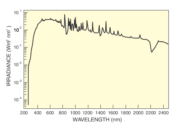
Most of our plots are linear plots. Log-lin plots are useful to illustrate the fall-off of the irradiance at the atmospheric edge because the log scale enhances the low value data and compresses the high value data. Plotting Figure 1 as a log-lin plot makes the entire spectrum look flatter as the peaks are reduced. When two plots, such as solar and simulator irradiance are both plotted on the same log-lin grid, differences appear less.

Convenient definitions of spectral regions include UVA, UVB, UVC, visible and infrared, (also sometimes divided into IR-A and IR-B). The exact boundaries of these regions remain the subject of debate.