Analysis of Optical Ray Paths in Spectrocopy Instruments

A simple case is shown in Figure 10-1. Light of wavelength λ enters the instrument through the entrance slit and diverges toward the grating, which diffracts the incident light into a number of orders {m} given by the grating equation (for all orders m for which β given by Eq. (2-1) is real). One of these orders (say m = 1) is the analytical order, that which is designed to pass through the exit slit. All other propagating orders, including the ever-present m = 0 order, are diffracted away from the exit slit and generally strike an interior wall of the instrument, which absorbs some of the energy, reflects some, and scatters some.

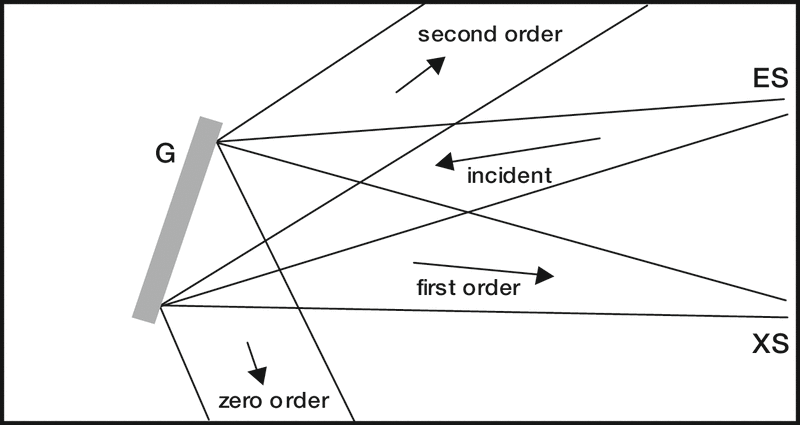
Some of the light reaching the interior walls may reflect or scatter directly toward the exit slit, but most of it does not; that which is reflected or scattered in any other direction will eventually reach another interior wall or it will return to the grating (and thereby be diffracted again).

This simple illustration allows us to draw a number of conclusions regarding the relative intensities of the various rays reaching the exit slit. We call E(λ,m) the diffraction efficiency of the grating (in this use geometry) at wavelength λ in order m; therefore, we choose a grating for which E(λ,1) is maximal in this use geometry (which will minimize the efficiencies of the other propagating orders: E(λ,0), E(λ,-1), etc.; see Section 9.12). We further call ε the fraction of light incident on an interior wall that is reflected and Φ the fraction that is scattered in any given direction, and stipulate that both ε and Φ are much less of unity (i.e., we have chosen the interior walls to be highly absorbing). [Generally, ε and Φ depend on wavelength and incidence angle, and Φ on the direction of scatter as well, but for this analysis we ignore these dependencies.]

With these definitions, we can approximate total intensity I(λ,1) of the light incident on the grating that reaches the exit slit when the system is tuned to transmits wavelength λ in order m = 1 as

Equation Coming Soon (10.2)

where I₀(λ) is the intensity incident on the grating and O(3) represents terms of order three or higher in ε and Φ.

The first term in Eq. (10-2) is the intensity in the analytical wavelength and diffraction order; in an ideal situation, this would be the only light passing through the exit slit, so we may call this quantity the “desired signal”. Subtracting this quantity from both sides of Eq. (10-2), dividing by it and collecting terms yields the fractional stray light S(λ,1):

Equation Coming Soon (10.3)

The first term in Eq. (10-3) is the sum, over all other propagating orders, of the fraction of light in those diffracted orders that is reflected by an interior wall to the exit slit, divided by the desired signal; each element in this sum is generally zero unless that order strikes the wall at the correct angle. The second term is the sum, over all other orders, of the fraction of light in those orders that is scattered directly into the exit slit; the elements in this sum are generally nonzero, again divided by the desired signal. Both of these sums are linear in ε or Φ (both << 1) and in E(λ,m≠1) (each of which is considerably smaller than E(λ,1) since we have chosen the grating to be blazed in the analytical order). The third through fifth sums represent light that is reflected off two walls into the exit slit, or scattered off two walls into the exit slit, or reflected off one wall and scattered off another wall to reach the exit slit – in all three cases, the terms are quadratic in either ε or Φ and can therefore be neglected (under our assumptions).

If we generalize this analysis for a broad-spectrum source, so that wavelengths other than λ are diffracted by the grating, then we obtain

Equation Coming Soon (10.4)

Note that, in each term, the integral over wavelength is inside the sum, since the upper limit of integration is limited by the grating equation (2-1) for each diffraction order m. Of course, the integration limits may be further restricted if the detector employed is insensitive in certain parts of the spectrum.