Optics Formulas
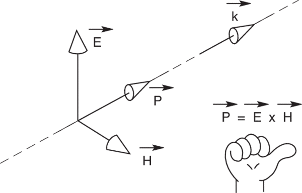
Light Right-Hand Rule
Light is a transverse electromagnetic wave. The electric E and magnetic M fields are perpendicular to each other and to the propagation vector k, as shown below.
Power density is given by Poynting’s vector, P, the vector product of E and H. You can easily remember the directions if you “curl” E into H with the fingers of the right hand: your thumb points in the direction of propagation.
Intensity Nomogram
The nomogram below relates E, H, and the light intensity I in vacuum. You may also use it for other area units, for example, [V/mm], [A/mm] and [W/mm2]. If you change the electrical units, remember to change the units of I by the product of the units of E and H: for example [V/m], [mA/m], [mW/m2] or [kV/m], [kA/m], [MW/m2].
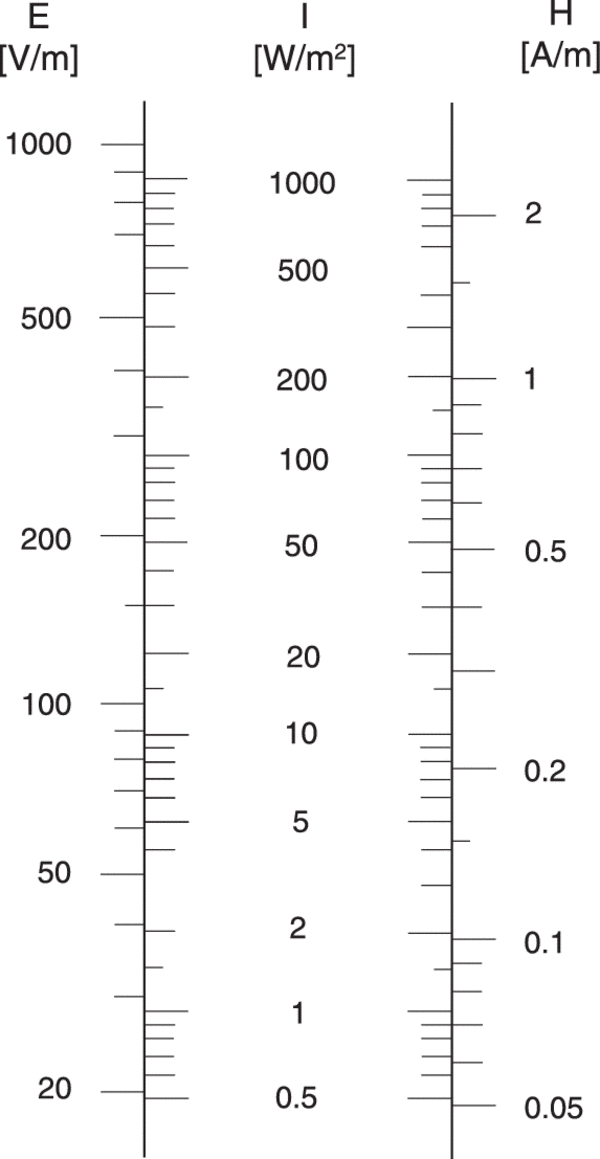
Light Intensity
The light intensity, I is measured in Watts/m2, E in Volts/m, and H in Amperes/m. The equations relating I to E and H are quite analogous to OHMS LAW. For peak values these equations are:
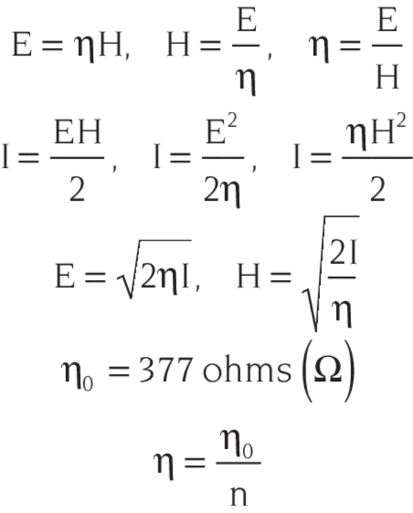
The quantity η0 is the wave impedance of vacuum, and η is the wave impedance of a medium with refractive index n.
Wave Quantity Relationship
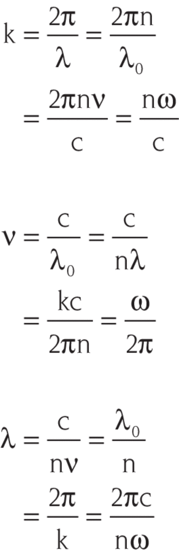
- k: wave vector [radians/m]
- ν: frequency [Hertz]
- ω: angular frequency [radians/sec]
- λ: wavelength [m]
- λ0: wavelength in vacuum [m]
- n: refractive index
Light Energy Conversions
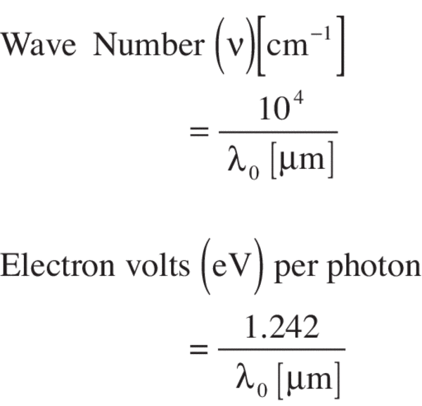
Wavelength Conversions
1 nm = 10 Angstroms (Å) = 10-9 m = 10-7 cm = 10-3 µm
Plane-Polarized Light
For plane-polarized light the E and H fields remain in perpendicular planes parallel to the propagation vector k, as shown below.
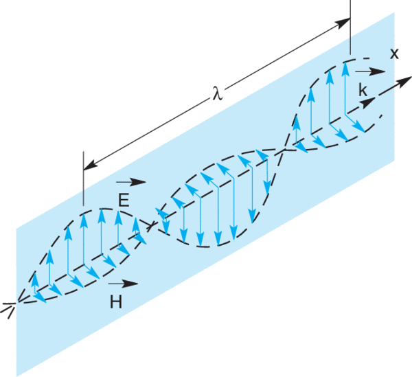
Both E and H oscillate in time and space as: sin (ωt-kx)
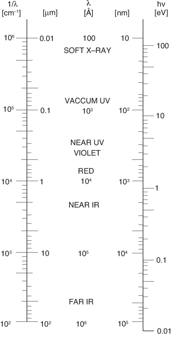
Wavelength Nomogram
The wavelength nomogram relates wavenumber, photon energy and wavelength.
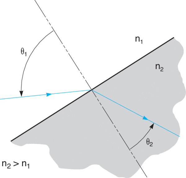
Snell’s Law
Snell’s Law describes how a light ray behaves when it passes from a medium with index of refraction n1, to a medium with a different index of refraction, n2. In general, the light will enter the interface between the two media at an angle. This angle is called the angle of incidence. It is the angle measured between the normal to the surface (interface) and the incoming light beam (see figure). In the case that n1 is smaller than n2, the light is bent towards the normal. If n1 is greater than n2, the light is bent away from the normal (see figure below). Snell’s Law is expressed as n1sinθ1 = n2sinθ2.
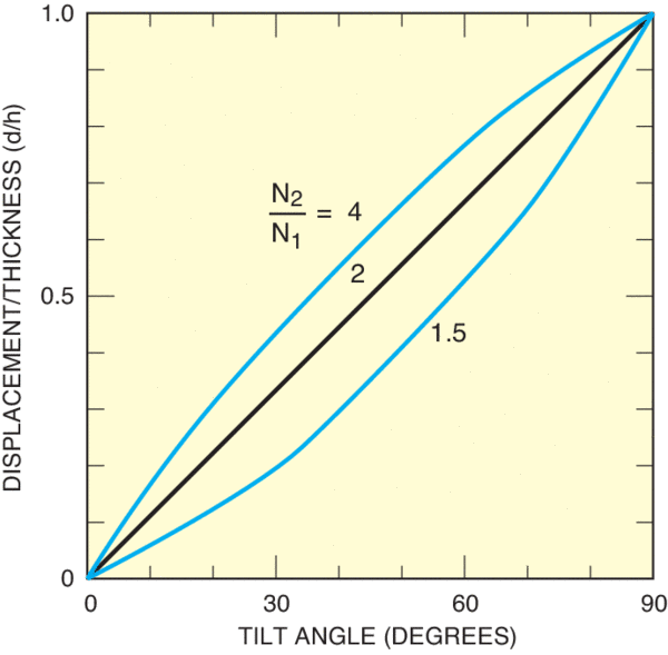
Beam Displacement
A flat piece of glass can be used to displace a light ray laterally without changing its direction. The displacement varies with the angle of incidence; it is zero at normal incidence and equals the thickness h of the flat at grazing incidence.
Grazing incidence is light incident at almost or close to 90° to the normal of the surface.
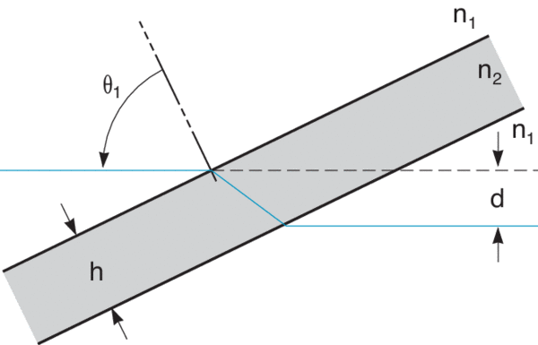
The relationship between the tilt angle of the flat and the two different refractive indices is shown in the graph below.
Beam Deviation
Both displacement and deviation occur if the media on the two sides of the tilted flat are different — for example, a tilted window in a fish tank. The displacement is the same, but the angular deviation δ is given by the formula below. Note:δ is independent of the index of the flat; it is the same as if a single boundary existed between media 1 and 3. (see Figure 9)
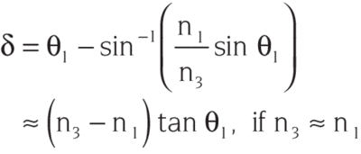
Example: The refractive index of air at STP (Standard Temperature and Pressure) is about 1.0003. The deviation of a light ray passing through a glass Brewster’s angle window on a HeNe laser is then:
δ= (n3 - n1) tan θ
At Brewster’s angle, tan θ= n2
δ= (0.0003) x 1.5 = 0.45 mrad
At 10,000 ft. altitude, air pressure is 2/3 that at sea level; the deviation is 0.30 mrad. This change may misalign the laser if its two windows are symmetrical rather than parallel.
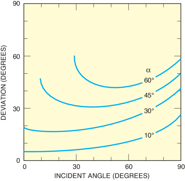
Angular Deviation of a Prism
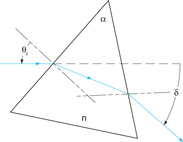
Angular deviation of a prism depends on the prism angle α, the refractive index, n, and the angle of incidence θi. Minimum deviation occurs when the ray within the prism is normal to the bisector of the prism angle. For small prism angles (optical wedges), the deviation is constant over a fairly wide range of angles around normal incidence. For such wedges the deviation is:
δ ≈ (n - 1)α
Prism Total Internal Reflection (TIR)
TIR depends on a clean glass-air interface. Reflective surfaces must be free of foreign materials. TIR may also be defeated by decreasing the incidence angle beyond a critical value. For a right angle prism of index n, rays should enter the prism face at an angle θ:
θ < arcsin (((n2-1)1/2-1)/√2)
In the visible range, θ = 5.8° for BK 7 (n = 1.517) and 2.6° for fused silica (n = 1.46). Finally, prisms increase the optical path. Although effects are minimal in laser applications, focus shift and chromatic effects in divergent beams should be considered.
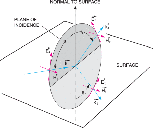
Fresnel Equations:
- i - incident medium
- t - transmitted medium
use Snell’s law to find θt
Normal Incidence:
r = (ni-nt)/(ni + nt)
t = 2ni/(ni + nt)
Brewster's Angle:
θβ = arctan (nt/ni)
Only s-polarized light reflected.
Total Internal Reflection (TIR):
θTIR > arcsin (nt/ni)
nt < ni is required for TIR
Field Reflection and Transmission Coefficients:
The field reflection and transmission coefficients are given by:
r = Er/Ei t = Et/Ei
Non-Normal Incidence:
rs = (nicosθi -ntcosθt)/(nicosθi + ntcosθt)
rp = (ntcos θi -nicosθt)/ntcosθi + nicosθt)
ts = 2nicosθi/(nicosθi + ntcosθt)
tp = 2nicosθi/(ntcosθi + nicosθt)
Power Reflection:
The power reflection and transmission coefficients are denoted by capital letters:
R = r2 T = t2(ntcosθt)/(nicosθi)
The refractive indices account for the different light velocities in the two media; the cosine ratio corrects for the different cross sectional areas of the beams on the two sides of the boundary.
The intensities (watts/area) must also be corrected by this geometric obliquity factor:
It = T x Ii(cosθi/cosθt)
Conservation of Energy:
R + T = 1
This relation holds for p and s components individually and for total power.
Polarization
To simplify reflection and transmission calculations, the incident electric field is broken into two plane-polarized components. The “wheel” in the pictures below denotes plane of incidence. The normal to the surface and all propagation vectors (ki, kr, kt) lie in this plane.
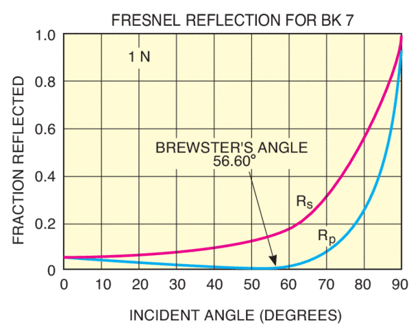
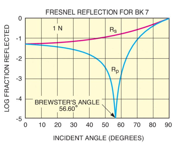
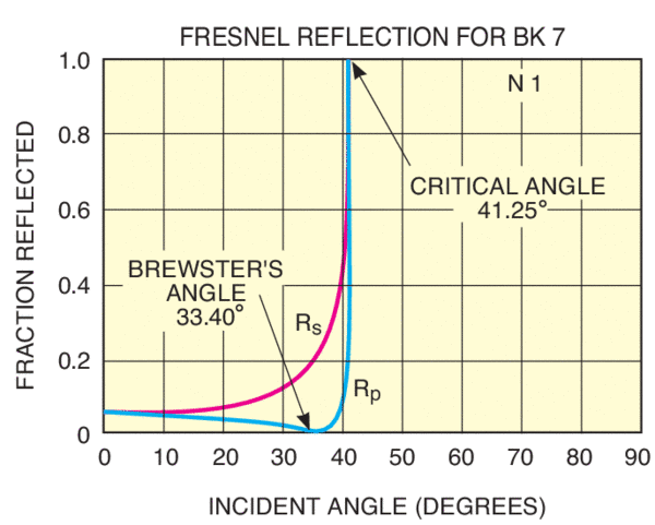
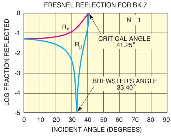
Power Reflection Coefficients
Power reflection coefficients Rs and Rp are plotted linearly and logarithmically for light traveling from air (ni = 1) into BK 7 glass (nt = 1.51673). Brewster’s angle = 56.60°.
The corresponding reflection coefficients are shown below for light traveling from BK 7 glass into air Brewster’s angle = 33.40°. Critical angle (TIR angle) = 41.25°.
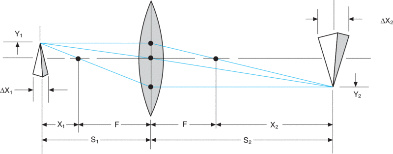
Thin Lens Equations
If a lens can be characterized by a single plane then the lens is “thin”. Various relations hold among the quantities shown in the figure 15.
Gaussian:
1/s1 + 1/s2 = 1/F
Newtonian:
x1x2 = -F2
Transverse Magnification:
MT = Y2/Y1 = -S2/S1
MT < 0, image inverted
Longitudinal Magnification:
ML = ΔX2/ΔX1 = -MT2
ML <0, no front to back inversion
Sign Conventions for Images and Lenses
| Quantity | + | - |
| s1 | real | virtual |
| s2 | real | virtual |
| F | convex lens | concave lens |
Lens Types for Minimum Aberration
| | s2/s1 | | Best lens |
| <0.2 | plano-convex/concave |
| >5 | plano-convex/concave |
| >0.2 or <5 | bi-convex/concave |
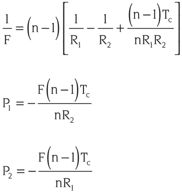
Thick Lenses
A thick lens cannot be characterized by a single focal length measured from a single plane. A single focal length F may be retained if it is measured from two planes, H1, H2, at distances P1, P2 from the vertices of the lens, V1, V2. The two back focal lengths, BFL1 and BFL2, are measured from the vertices. The thin lens equations may be used, provided all quantities are measured from the principal planes.

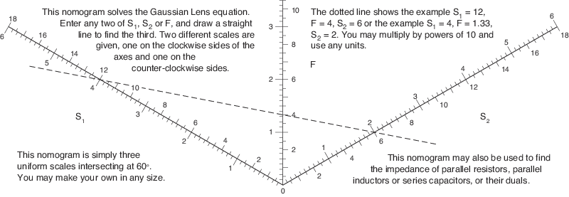
Lens Nomogram:
The Lensmaker’s Equation
Convex surfaces facing left have positive radii. Below, R1>0, R2<0. Principal plane offsets, P, are positive to the right. As illustrated, P1>0, P2<0. The thin lens focal length is given when Tc = 0.
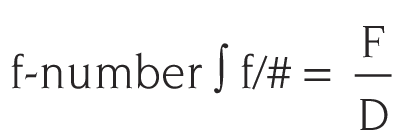
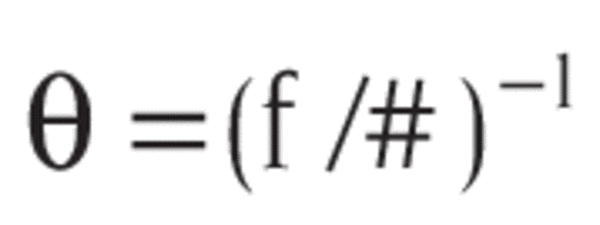
Numerical Aperture
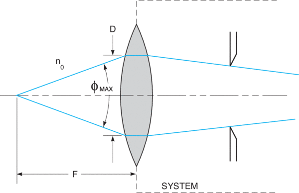
φMAX is the full angle of the cone of light rays that can pass through the system.
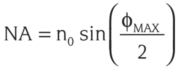
For small φ:
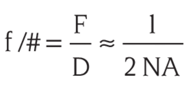
Both f-number and NA refer to the system and not the exit lens.
Constants and Prefixes
| Speed of light in vacuum | c = 2.998 x 10⁸ m/s |
| Planck’s const. | h = 6.625 x 10⁻³⁴ Js |
| Boltzmann’s const. | k = 1.308 x 10⁻²³ J/K |
| Stefan-Boltzmann | σ = 5.67 x 10⁻⁸ W/m2K4 |
| 1 electron volt | eV = 1.602 x 10⁻¹⁹ J |
| exa (E) | 1018 |
| peta (P) | 1015 |
| tera (T) | 1012 |
| giga (G) | 109 |
| mega (M) | 106 |
| kilo (k) | 103 |
| milli (m) | 10-3 |
| micro (µ) | 10-6 |
| nano (n) | 10-9 |
| pico (p) | 10-12 |
| femto (f) | 10-15 |
| atto (a) | 10-18 |
Wavelengths of Common Lasers
| Source | (nm) |
|---|---|
| ArF | 193 |
| KrF | 248 |
| Nd:YAG(4) | 266 |
| XeCl | 308 |
| HeCd | 325, 441.6 |
| N2 | 337.1, 427 |
| XeF | 351 |
| Nd:YAG(3) | 354.7 |
| Ar | 488, 514.5, 351.1, 363.8 |
| Cu | 510.6, 578.2 |
| Nd:YAG(2) | 532 |
| HeNe | 632.8, 543.5, 594.1, 611.9, 1153, 1523 |
| Kr | 647.1, 676.4 |
| Ruby | 694.3 |
| Nd:Glass | 1060 |
| Nd:YAG | 1064, 1319 |
| Ho:YAG | 2100 |
| Er:YAG | 2940 |
Gaussian Intensity Distribution
The Gaussian intensity distribution:
I(r) = I(0) exp(-2r2/ω02)
is shown below
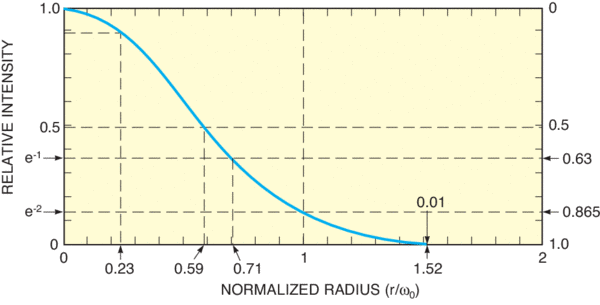
The right hand ordinate gives the fraction of the total power encircled at radius r:
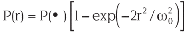
The total beam power, P(∞) [watts], and the on-axis intensity I(0) [watts/area] are related by:
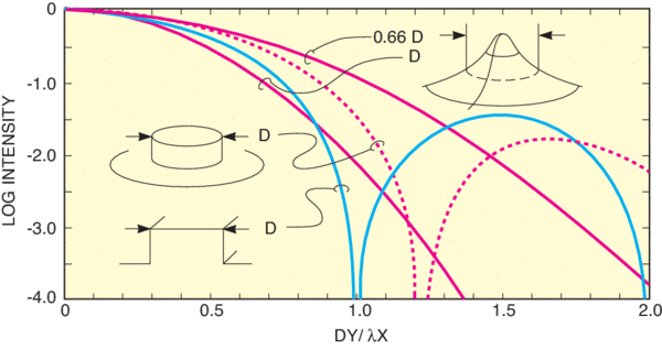
Diffraction
Figure 25 below compares the far-field intensity distributions of a uniformly illuminated slit, a circular hole, and Gaussian distributions with 1/e2 diameters of D and 0.66D (99% of a 0.66D Gaussian will pass through an aperture of diameter D). The point of observation is Y off axis at a distance X>>Y from the source.
Focusing a Collimated Gaussian Beam
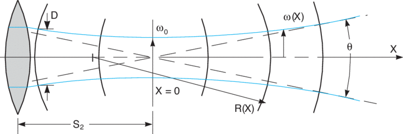
In the figure 26 above the 1/e2 radius, ω(x), and the wavefront curvature, R(x), change with x through a beam waist at x = 0. The governing equations are:
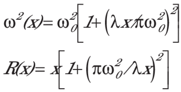
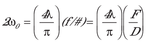
2ω0 is the waist diameter at the 1/e2 intensity points. The wavefronts are planar at the waist [R(0) = ∞].
At the waist, the distance from the lens will be approximately the focal length: s2 ≈ F.
D = collimated beam diameter or diameter illuminated on lens.
Depth of Focus (DOF)
DOF = (8λ/π)(f/#)2
Only if DOF < F, then
New Waist Diameter
Beam Spread
Optical Density
D = - log (T)
or
T= 10-D
SAG
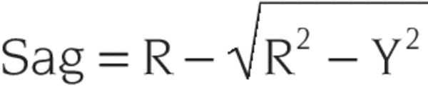
where R = radius of curvature and Y = radius of the aperture of the surface. SAG is an abbreviation for "sagitta," the Latin word for arrow. Used to specify the distance on the normal from the surface of a concave lens to the center of the curvature. It refers to the height of a curve measured from the chord.