Spectroscopy Instrument Imaging

The image of the entrance slit, ignoring aberrations and the diffraction limit, will not have the same dimensions as the entrance slit itself. Calling w and h the width and height of the entrance slit, and w' and h' the width and height of its image, the tangential and sagittal magnifications xT and xS are

xT ≡ w'/w = r'cosα/rcosβ, xS ≡ h'/h = r'/r (8-2)

These relations, which indicate that the size of the image of the entrance slit will usually differ from that of the entrance slit itself, are derived below.

Figure 8-3 shows the plane of dispersion. The grating center is at O; the x-axis is the grating normal and the y-axis is the line through the grating center perpendicular to the grooves at O. Monochromatic light of wavelength λ leaves the entrance slit (of width w) located at the polar coordinates (r, α) from the grating center O and is diffracted along angle β. When seen from O, the entrance slit subtends an angle Δα in the

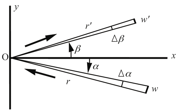
dispersion (xy) plane. Rays from one edge of the entrance slit have incidence angle α, and are diffracted along β; rays from the other edge have incidence angle α + Δα, and are diffracted along β – Δβ.* The image (located a distance r' from O), therefore subtends an angle Δβ when seen from O, has width w' = r'Δβ. The ratio xT = w'/w is the tangential magnification.

We may apply the grating equation to the rays on either side of the entrance slit:

Gmλ = sinα + sinβ    (8-3)

Gmλ = sin(α+Δα)+ sin(β–Δβ)    (8-4)

Here G (= 1/d) is the groove frequency along the y-axis at O, and m is the diffraction order. Expanding sin(α+Δα) in Eq. (8-4) in a Taylor series about Δα = 0, we obtain

sin(α+Δα) = sinα + (cosα)Δα + ...    (8-5)

where terms of order two or higher in Δα have been truncated. Using Eq. (8-5) (and its analogue for sin(β–Δβ)) in Eq. (8-4), and subtracting it from Eq. (8-3), we obtain

cosαΔα = cosβΔβ    (8-6)

and therefore

Δβ/Δα = cosα/cosβ    (8-7)

from which the first of Eqs. (8-2) follows.

Figure 8-4 shows the same situation in the sagittal plane, which is perpendicular to the principal plane and contains the pole diffracted ray. The entrance slit is located below the principal plane; consequently, its image is above this plane. A ray from the top of the center of the entrance slit is shown. Since the grooves are parallel to the sagittal plane at O, the grating acts as a mirror in this plane, so the angles Φ and Φ' are equal in magnitude.

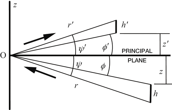
Ignoring signs, the tangents of these angles are equal as well:

tanΦ = tanΦ' →  z/r = z'/r'    (8-8)

where z and z' are the distances from the entrance and exit slit points to the principal plane. A ray from an entrance slit point a distance |z + h| from this plane will image toward a point |z' + h'| from this plane, where h' now defines the height of the image. As this ray is governed by reflection as well,

tanΨ = tanΨ' → (z+h)/r = (z'+h')/r'   (8-9)

Simplifying this using Eq. (8-8) yields the latter of Eqs. (8-2).

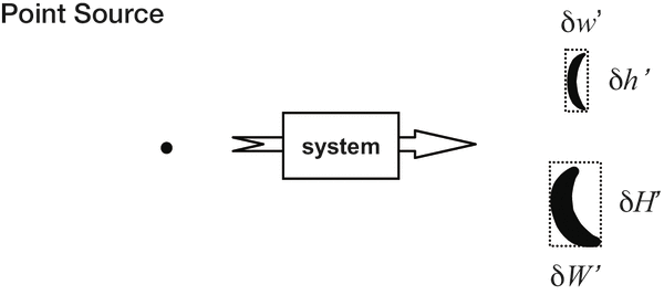
Consider a spectrometer with a point source located in the principal plane: the aberrated image of this point source has width δw' (in the dispersion direction) and height δh' (see Figure 8-5). If the point source is located out of the principal plane, it will generally be distorted, tilted and enlarged: its dimensions are now δW' and δH'. Because a point source is considered, these image dimensions are not due to any magnification effects of the system.

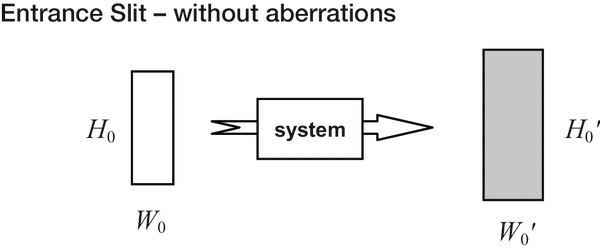
Now consider a rectangular entrance slit of width W₀ (in the dispersion plane) and height H₀. If we ignore aberrations and line curvature for the moment, we see that the image of the entrance slit is also a rectangle, whose width W₀' and height H₀' are magnified:

W₀' = xTW₀, H₀' = xSH₀    (8-10)

(see Figure 8-6).

Combining these two cases provides the following illustration (Figure 8-7). From this figure, we can estimate the width W' and height H' of the image of the entrance slit, considering both magnification effects and aberrations, as follows:

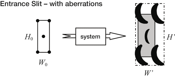
W' = xT W₀ + δW' = r'cosα/rcosβ W₀+ δW'    (8-11a)

H' = xS H₀ + δH' = r/r' H₀ + δH'    (8-11b)

Eqs. (8-11) allow the imaging properties of a grating system with an entrance slit of finite area to be estimated quite well from the imaging properties of the system in which an infinitesimally small object point is considered. In effect, rays need only be traced from one point in the en-trance slit (which determines δW' and δH'), from which the image dimensions for an extended entrance slit can be calculated using Eqs. (8-10).

The linespread function for a spectral image, as defined above, depends on the width of the exit aperture as well as on the width of the diffracted image itself. In determining the optimal width of the exit slit (or single detector element), a rule of thumb is that the width w" of the exit aperture should roughly match the width w' of the image of the entrance aperture, as explained below.

Typical linespread curves for the same diffracted image scanned by three different exit slit widths are shown in Figure 8-8. For simplicity, we have assumed xT = 1 for these examples. The horizontal axis is position along the image plane, in the plane of dispersion. This axis can also be thought of as a wavelength axis (that is, in spectral units); the two axes are related via the dispersion. The vertical axis is relative light intensity (or throughput) at the image plane; its bottom and top represent no intensity and total intensity (or no rays entering the slit and all rays entering the slit), respectively. Changing the horizontal coordinate represents scanning the monochromatic image by moving the exit slit across it, in the plane of dispersion. This is approximately equivalent to changing the wavelength while keeping the exit slit fixed in space.

An exit slit that is narrower than the image (w" < w') will result in a linespread graph such as that seen in Figure 8-8(a). In no position of the exit slit (or, for no diffracted wavelength) do all diffracted rays fall within the slit, as it is not wide enough; the relative intensity does not reach its maximum value of unity. In (b), the exit slit width matches the width of the image: w" = w'. At exactly one point during the scan, all of the diffracted light is contained within the exit slit; this point is the peak (at a relative intensity of unity) of the curve. In (c) the exit slit is wider than the image (w" > w'). The exit slit contains the entire image for many positions of the exit slit.

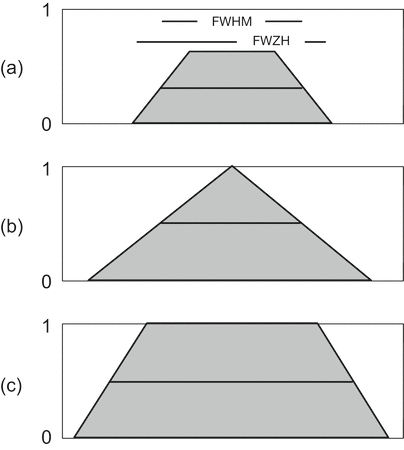
In these figures the quantities FWZH and FWHM are shown. These are abbreviations for full width at zero height and full width at half maximum. The FWZH is simply the total extent of the linespread function, usually expressed in spectral units. The FWHM is the spectral extent between the two extreme points on the linespread graph that are at half the maximum value. The FWHM is often used as a quantitative measure of image quality in grating systems; it is often called the effective spectral bandwidth. The FWZH is sometimes called the full spectral bandwidth. It should be noted that the terminology is not universal among authors and sometimes quite confusing.

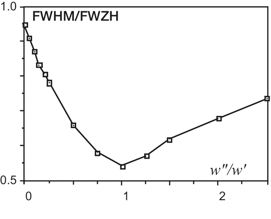
As the exit slit width w' is decreased, the effective bandwidth will generally decrease. If w' is roughly equal to the image width w, though, further reduction of the exit slit width will not reduce the bandwidth appreciably. This can be seen in Figure 8-8, in which reducing w' from case (c) to case (b) results in a decrease in the FWHM, but further reduction of w' to case (a) does not reduce the FWHM. The situation in w" < w' is undesirable in that diffracted energy is lost (the peak relative intensity is low) since the exit slit is too narrow to collect all the diffracted light at once. The situation w" > w' is also undesirable, since the FWHM is excessively large (or, similarly, an excessively wide band of wavelengths is accepted by the wide slit). The situation w" = w' seems optimal: when the exit slit width matches the width of the spectral image, the relative intensity is maximized while the FWHM is minimized. An interesting curve is shown in Figure 8-9, in which the ratio FWHM/FWZH is shown vs. the ratio w"/w' for a typical grating system. This ratio reaches its single minimum near w" = w'.

The height of the exit aperture has a more subtle effect on the imaging properties of the spectrometer, since by 'height' we mean extent in the direction perpendicular to the plane of dispersion. If the exit slit height is less than the height (sagittal extent) of the image, some diffracted light will be lost, as it will not pass through the aperture. Since diffracted images generally display curvature, truncating the sagittal extent of the image by choosing a short exit slit also reduces the width of the image. This latter effect is especially noticeable in Paschen-Runge mounts.

In this discussion we have ignored the diffraction effects of the grating aperture: the comments above consider only the effects of geometrical optics on instrumental imaging. For cases in which the entrance and exit slits are equal in width, and this width is two or three times the diffraction limit, the linespread function is approximately Gaussian in shape rather than the triangle shown in Figure 8-8(b).