Motion Control Theory Terminology
Common motion systems use three types of control methods. They are position control, velocity control and torque control. The majority of Newport’s motion systems use position control. This type of control moves the load from one known fixed position to another known fixed position. Feedback, or closed-loop positioning, is important for precise positioning. Velocity control moves the load continuously for a certain time interval or moves the load from one place to another at a prescribed velocity. Newport’s systems use both encoder and tachometer feedback to regulate velocity. Torque control measures the current applied to a motor with a known torque coefficient in order to develop a known constant torque.
Following Error
Following Error is the instantaneous difference between actual position as reported by the position feedback device and the ideal position, as commanded by the motion controller.
Settling Time
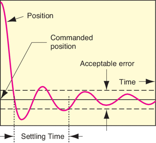
Settling Time is the amount of time elapsed between when a motorized stage first reaches a commanded position and when it maintains the commanded position to within an acceptable pre-defined error value (see Figure 1).
Overshoot
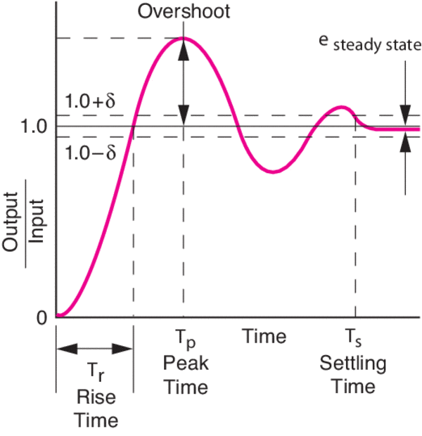
Overshoot is the amount of over-correction in an under-damped control system (see Figure 2).
Steady-State Error
Steady-State Error is the difference between actual and commanded position after the controller has finished applying corrections (see Figure 2 Above). As can be seen in the above figure, the commanded position is 1.0, however there is a small steady-state error after the position correction loop has completed.
Vibration
When the operating speed approaches a natural frequency of the mechanical system, structural vibrations, or ringing, can be induced. Ringing can also occur in a system following a sudden change in velocity or position. This oscillation will lessen the effective torque and may result in loss of synchronization between the motor and controller.
Settling times and vibrations can best be dealt with by damping motor oscillations through mechanical means such as friction or a viscous damper. When operating a stepper system, some additional methods that can change resonance vibration frequencies are:
- Half stepping or microstepping the motor
- Changing the system inertia
- Accelerating through the resonance speed ranges
- Modifying drivetrain torsional stiffness
In order to achieve smooth high-speed motion without over-taxing the motor, the controller must direct the motor driver to change velocity judiciously to achieve optimum results. This is accomplished using shaped velocity profiles to limit the accelerations and decelerations required.
Trapezoidal Profile
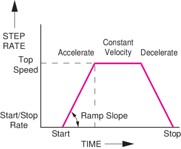
The trapezoidal profile changes velocity in a linear fashion until the target velocity is reached. When decelerating, the velocity again changes in a linear manner until it reaches zero velocity. Graphing velocity versus time results in a trapezoidal plot (see Figure 3). Advanced controllers allow user modification of the acceleration/deceleration with more advanced controllers allowing individual settings for acceleration and deceleration.
S Curve Profile
A trapezoidal velocity profile is adequate for most applications. Its only disadvantage is that it may cause some system disturbances at the “corners” that translate in small vibrations, which extend the settling time. For demanding applications sensitive to this phenomenon, the velocity profile can be modified to have an S shape during the acceleration and deceleration periods. This minimizes the vibrations caused in a mechanical system by a moving mass.
Open-Loop Control
Open-loop refers to a control technique that does not measure and act upon the output of the system. Most piezoelectric systems and inexpensive micrometer-replacement actuators are open-loop devices.
Open-loop positioners are useful when remote control is desired for improved accessibility or to avoid disturbing critical components by touching them.
Stepper and ministepper motors often use open-loop as well. The count of pulses is a good indicator of position but can be unpredictable unless loads, accelerations, and velocities are well known. Skipped or extra steps are frequent problems if the system is not properly designed.
Open-loop motion control has become very popular. Advances in ministepping technology and incorporation of viscous motor-damping mechanisms have greatly improved the positioning dependability and reduced vibration levels of today’s highest quality stepper devices.
Open-loop is by no means a synonym for crude. Even inexpensive open-loop devices can achieve very fine incremental motions. Nanometer-scale incremental motions are achievable by open-loop piezo-type devices.
Open-loop systems infer the approximate position of a motion device without using an encoder. In the case of a piezo device, the applied voltage is an indicator of position. However, the relationship is imprecise due to hysteresis and non-linearities inherent in commonplace piezo materials.
Closed-Loop Control
Closed-loop refers to a control technique that measures the output of the system compared to the desired input and takes corrective action to achieve the desired result. Electronic feedback mechanisms in closed-loop systems enhance the ability to correctly place and move loads.
Closed-Loop Control Techniques
Depending upon how the feedback signals are processed by the controller, different levels of performance can be achieved. The simplest type of feedback is called proportional control.
Other types are called derivative and integral control. Combining all three techniques into what is called PID control provides the best results.
Proportional Control
A control technique that multiplies the error signal (the difference between actual and desired position) by a user-specified gain factor Kp and uses it as a corrective signal to the motion system. The effective result is to exaggerate the error and react immediately to correct it.
Changes in position generally occur during commanded acceleration, deceleration, and in moves where velocity changes occur in the system dynamics during motion. As Kp is increased, the error is more quickly corrected. However, if Kp becomes too large, the mechanical system will begin to overshoot, and at some point, it may begin to oscillate, becoming unstable if it has insufficient damping.
Kp cannot completely eliminate errors; however, as the following error, e, approaches zero, the proportional correction element, Kpe, disappears. This results in some amount of steady-state error.
Integral Control
A control technique that accumulates the error signal over time, multiplies the sum by a user-specified gain factor Ki and uses the result as a corrective signal to the motion system. Since this technique also acts upon past errors, the correction factor does not go to zero as the following error, e, approaches zero allowing steady-state errors to be eliminated.
But the integral gain has an important negative side effect. It can be a destabilizing factor for the control loop. Large integral gains or integral gains used without proper damping could cause severe system oscillations. The contribution of integral gain to the control loop is limited by the integral saturation limit, Ks.
Derivative Control
A control technique that multiples the rate of change of the following error signal by a user-specified gain Kd and uses the result as a corrective signal to the motion system. Since this type of control acts to stabilize the transient response of a system, it may be thought of as electronic damping.
Increasing the value of Kd increases the stability of the system. The steady-state error, however, is unaffected since the derivative of the steady-state error is zero.
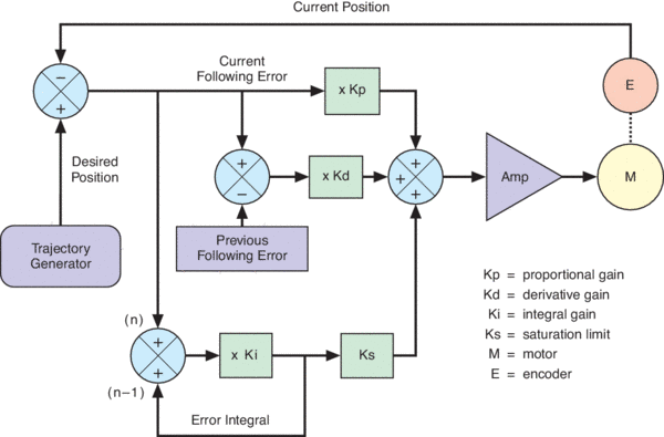
PID Control
The combination of proportional plus integral plus derivative control. For motion systems, the PID loop has become a very popular control algorithm (see Figure 4). The feedback elements are interactive, and knowing how they interact is essential for tuning a motion system. Optimum system performance requires that the coefficients, Kp, Ki, and Kd be tuned for a given combination of motion mechanics and payload inertias.
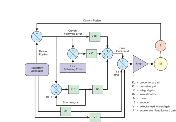
Feed Forward Loops
When using a PID control algorithm, an error between the desired and actual positions must exist in order to generate a corrective input. The implication of this is that there will always be some non-zero following error. The goal when using a feed forward loop is to minimize following error. The concept in using a feed forward loop is to predict how the system will function in future updates and to make corrections now based on those estimates (see Figure 5).
The corrections are generally implemented by multiplying the desired velocity with the velocity feed-forward gain factor Vf. The same technique can be used to apply an acceleration feed-forward correction signal. This correction is being used to reduce the average following error during the acceleration and deceleration periods.
Combining feed forward techniques with PID allows the PID loop to correct only for the residual error left by the feed forward loop, thereby improving overall system response.
Positioning Trajectory Options
Motion without Interpolation
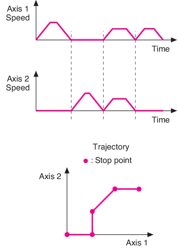
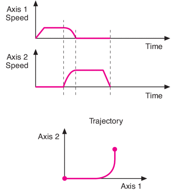
There are three types of non-interpolated motion: single-axis, simultaneous, and synchronized motion.
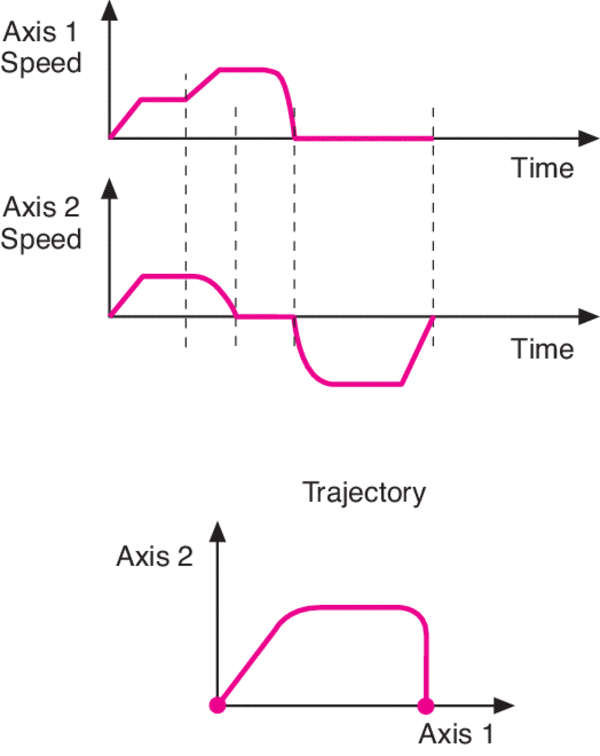
Simultaneous and synchronized motion are both multi-axis (see Figure 6).
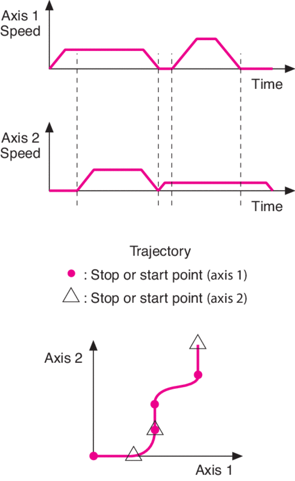
The difference between them is that simultaneous motion is unsynchronized (see Figure 7).
Motion with Interpolation
When the controlled load must follow a particular path to get from its starting point to its stopping point, the coordination of axis movements is said to be interpolated. There are two types of interpolation: linear and circular.
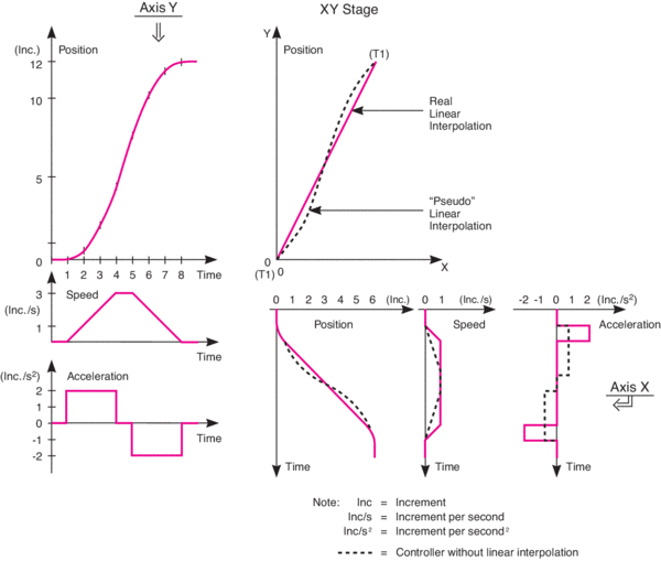
Linear Interpolation
Linear interpolation is required for multi-axis motion from one point to another in a straight line. The controller determines the speeds on each axis so that the movements are coordinated. True linear interpolation requires the ability to modify acceleration. Some controllers approximate linear interpolation using pre-calculated acceleration profiles (see Figure 8).
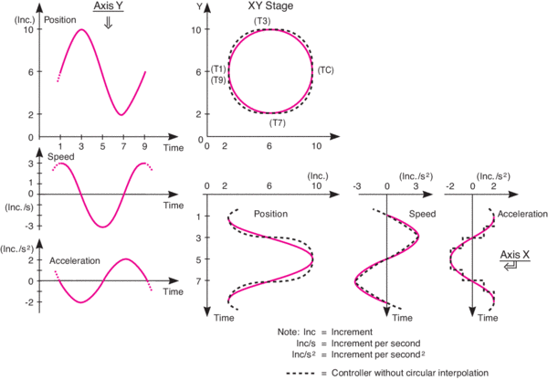
Circular Interpolation
Circular interpolation is the ability to move the payload around a circular trajectory.
It requires the controller to modify acceleration on the fly (see Figures 9 and 10).
Contouring
With contouring, the controller changes the speeds on the different axes so that the trajectories pass smoothly through a set of predefined points. The speed is defined along the trajectory and can be constant, except during starting and stopping (see Figure 11).