 Over 8,000 products in-stock! & FREE 2-Day shipping on all web orders!* Learn More FREE T-Shirt with orders $250+ Details
- Products
- Solutions
- Resources
-
Support
- Technical Support
- Service & Returns
- Trade Shows & Events
- Company Information
- About Newport
- Company Overview
- Trade Shows & Events
- Quality Commitments
- Careers
- Contacts & Locations
- Contact Us
- Corporate Headquarters
- Worldwide Sales & Service
- Supplier Information
- Supplier Code of Conduct
- Terms & Conditions of Purchase
-
Contact
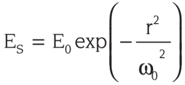
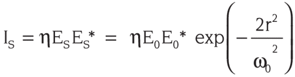
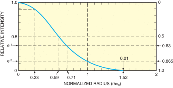
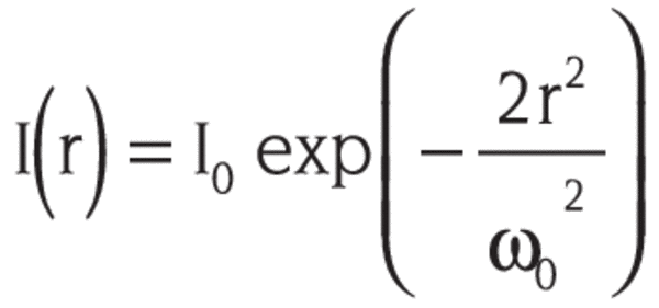
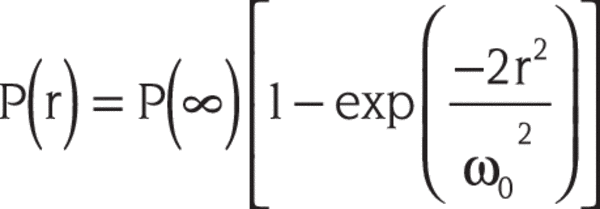
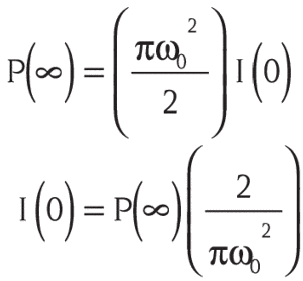
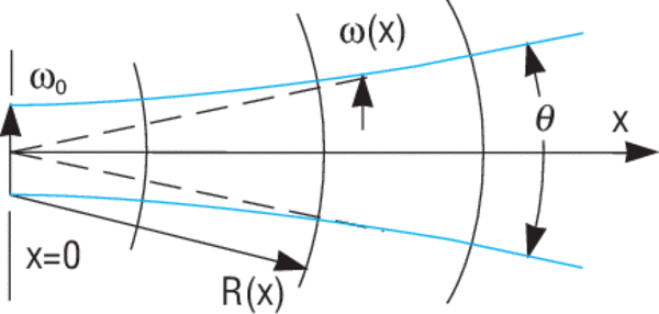
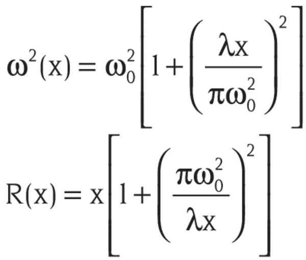
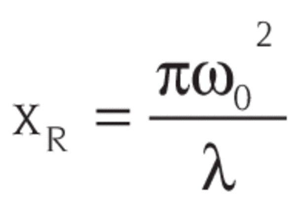
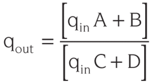
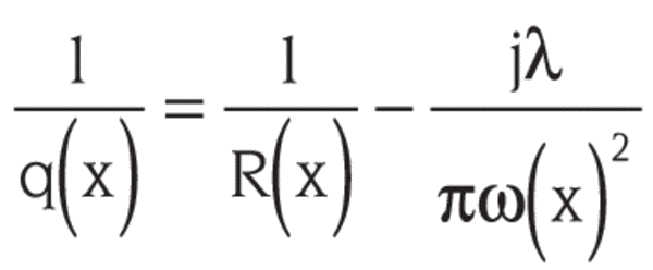
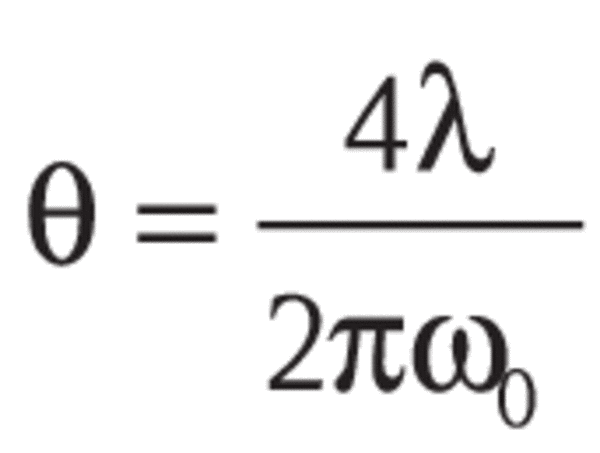
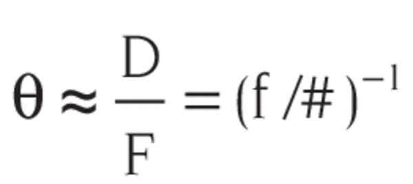
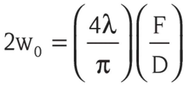
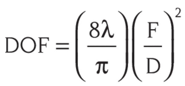
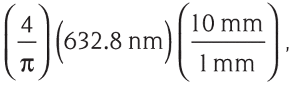
 Ultra-High Velocity